• Home
• Research
• Publications
• CV (pdf)
• Teaching
• Outreach

SMILER MATLAB Example: Saliency Calculations on Noisy Stimuli

1. Introduction
2. SMILER Setup
3. Example Experiment Setup
4. Experiment Walkthrough
5. Concluding Remarks

Images and code to run this example can be downloaded from this GitHub repository.

Introduction

This is an example which showcases how to use SMILER while operating in the MATLAB environment. Note that we highly recommend using the SMILER CLI in order to unlock the full potential of SMILER, as there are a number of models which are not supported through MATLAB (however, the with MATLAB Python API installed, the CLI supports all models included in SMILER).

Note that this exercise is designed purely as an example; the stimuli and experiment design have been selected to show an interesting use case for saliency models, but the size of the test is purposefully kept small to run in a reasonable amount of time. Any conclusions or judgements about algorithm performance are therefore tentative at best.

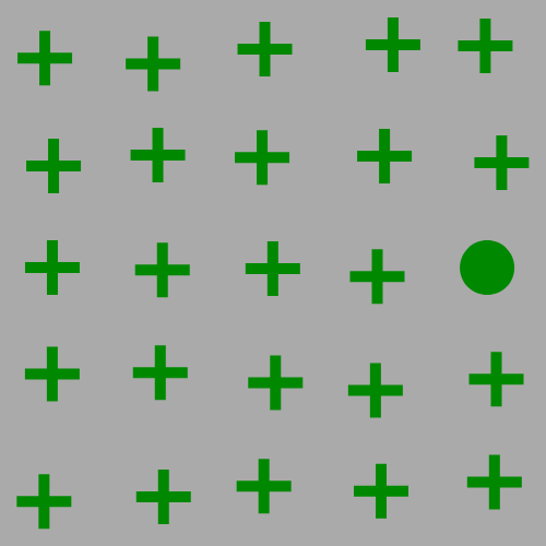
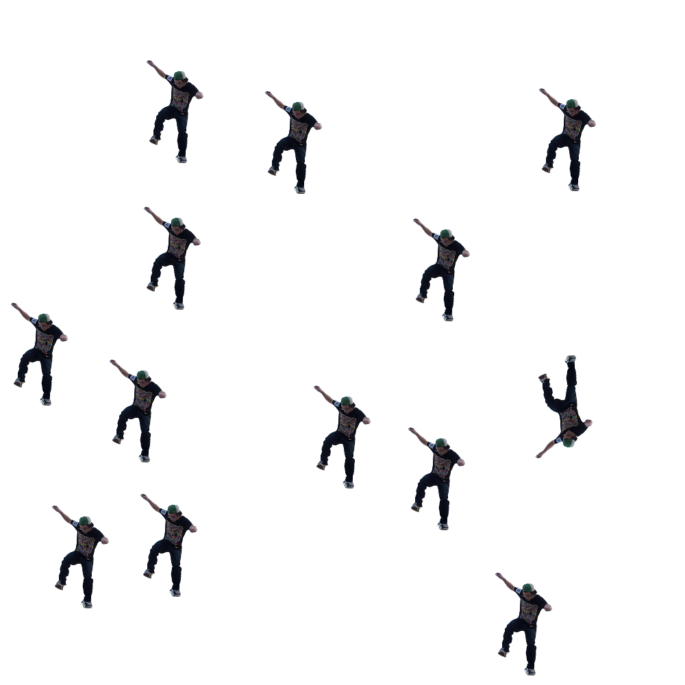
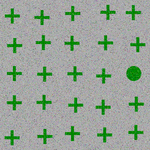
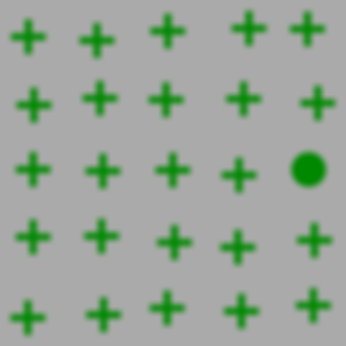
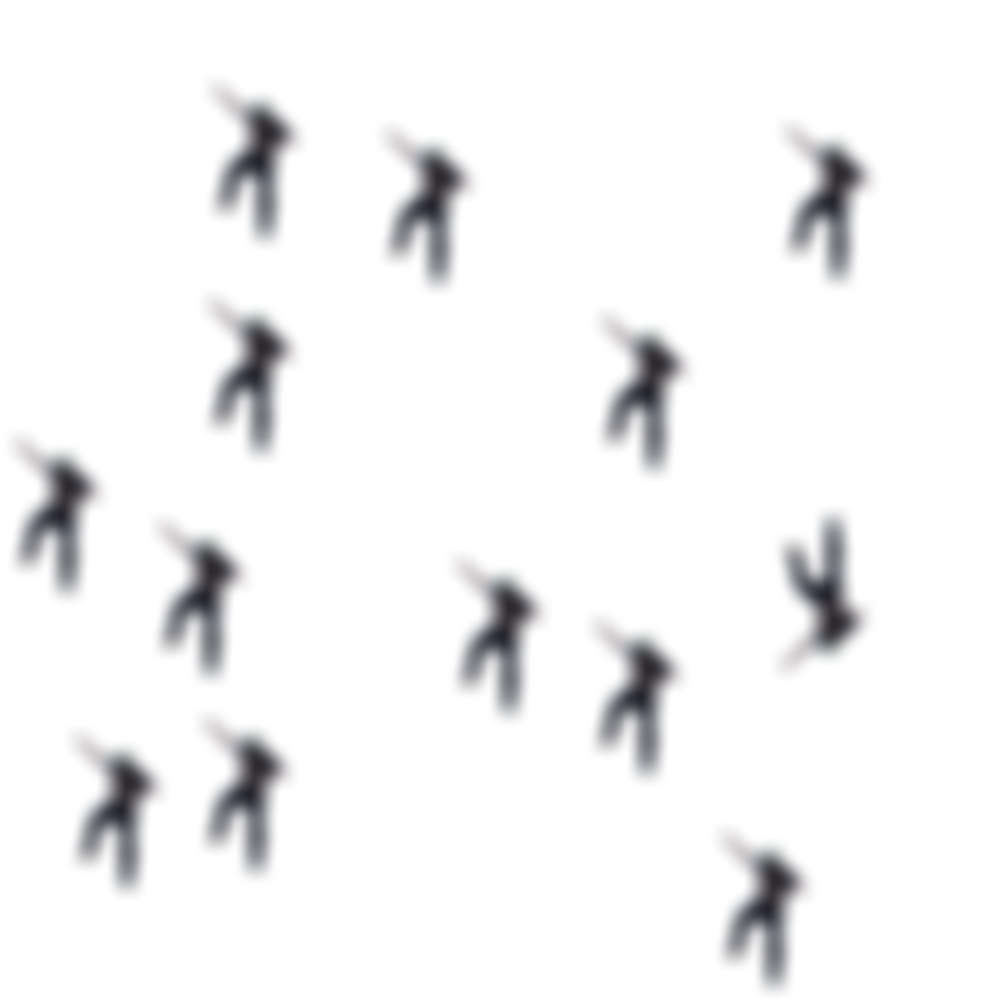
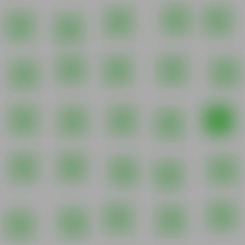
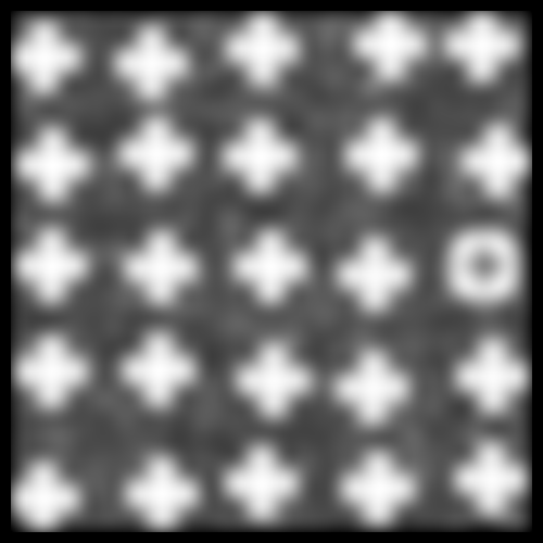
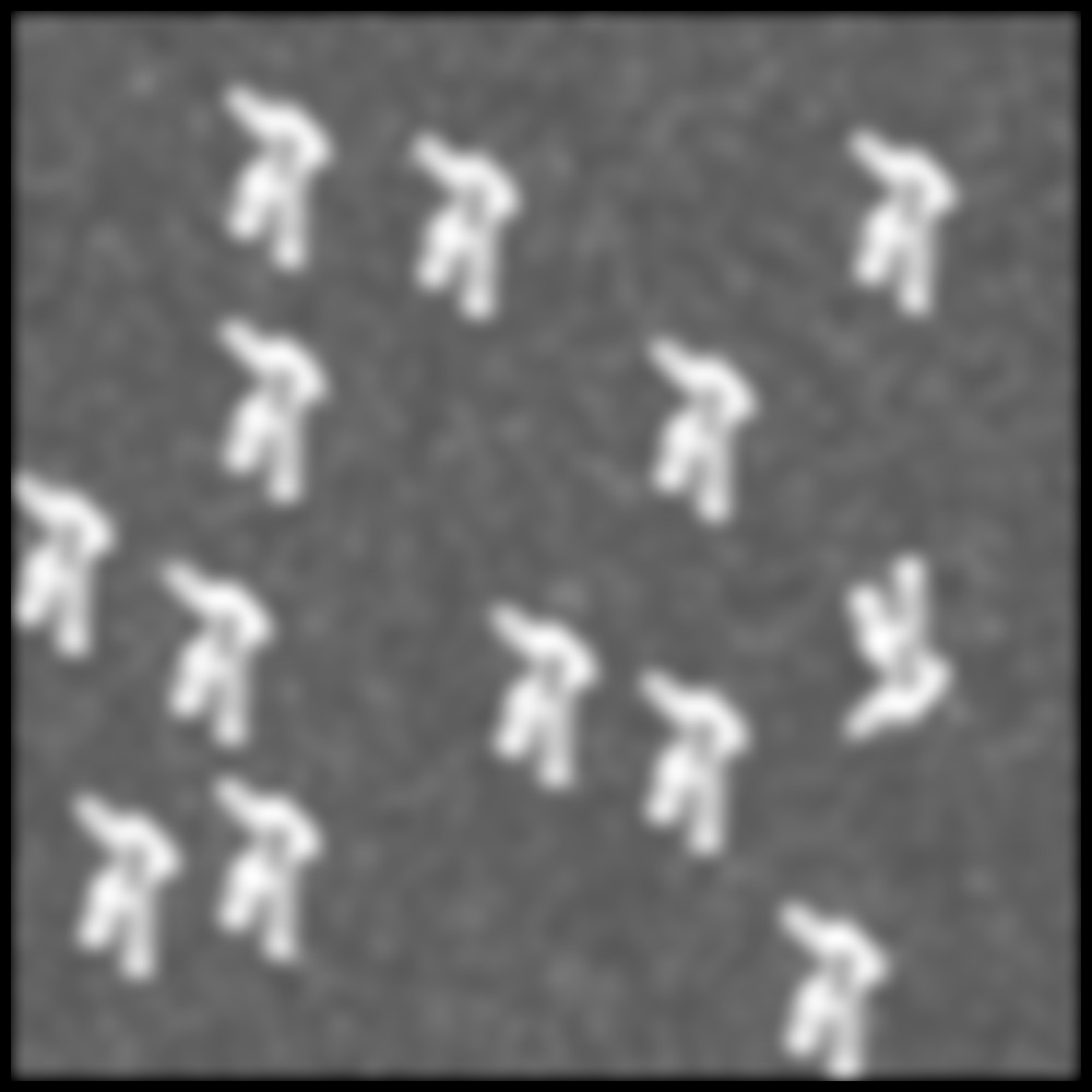
The focus of this example is on singleton search targets in psychophysical search arrays. Each search array contains a single unique target which contextually would be expected to be found to be more salient than other elements in the image. This experiment examines how this judgement of target salience changes with the addition of two types of noise: randomized point noise and blurring.

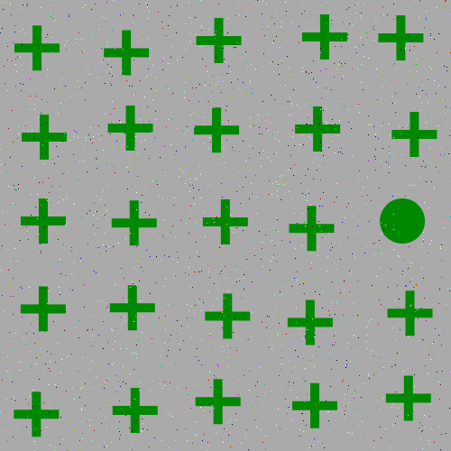
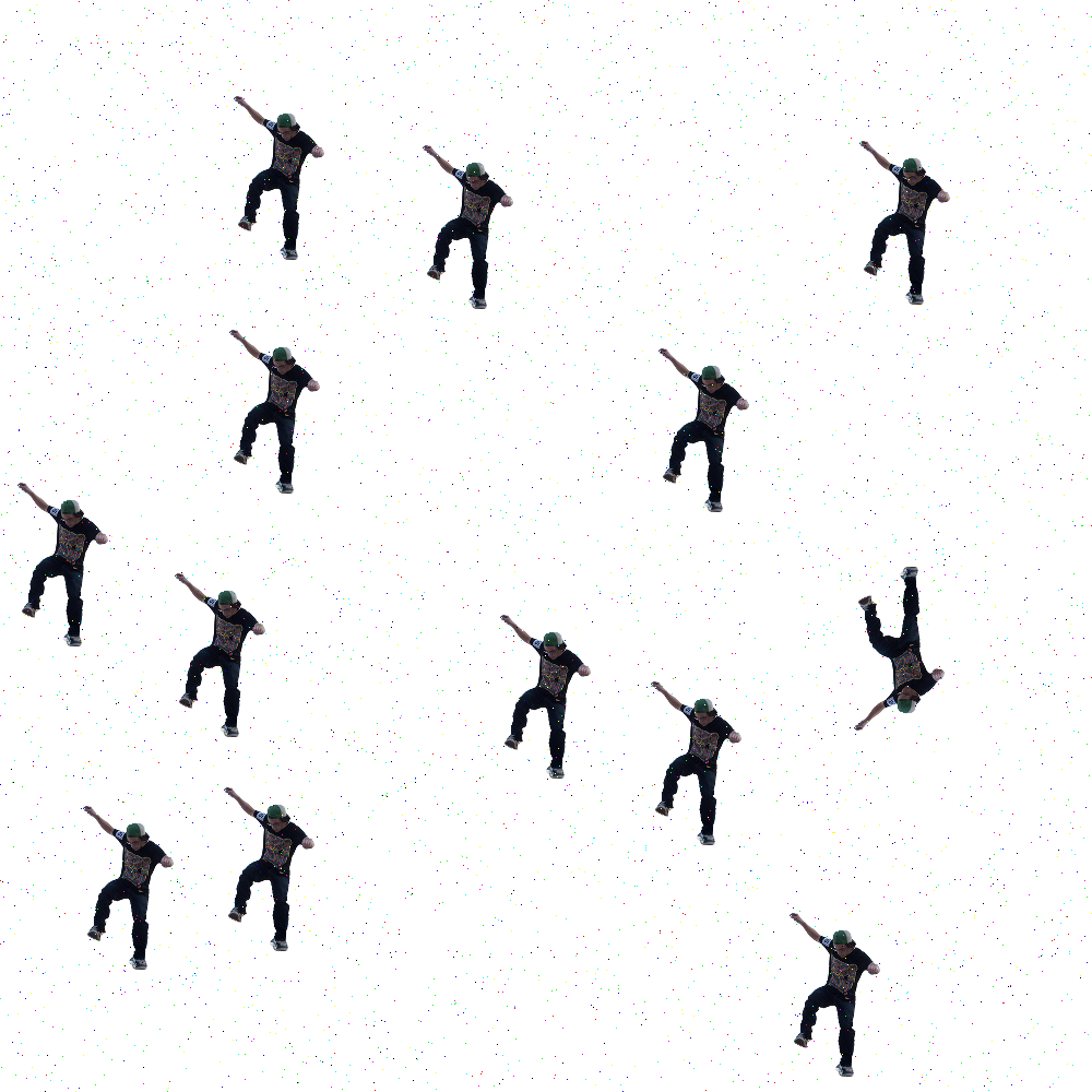
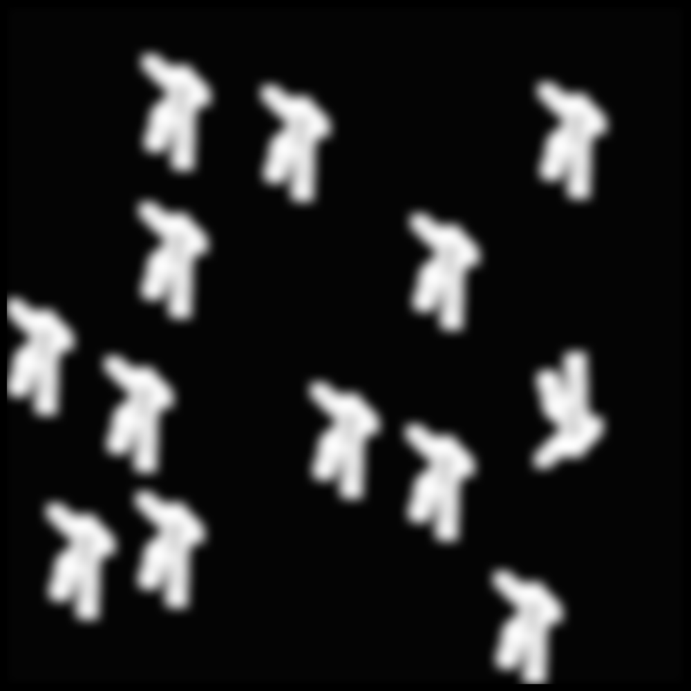
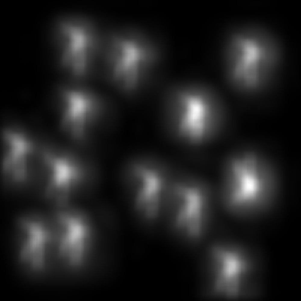
Here are the example stimuli under point noise degredation:

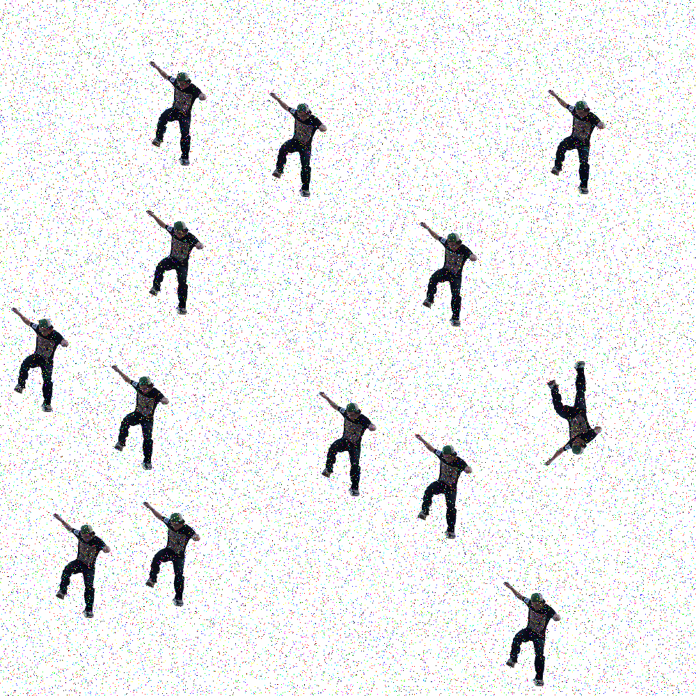
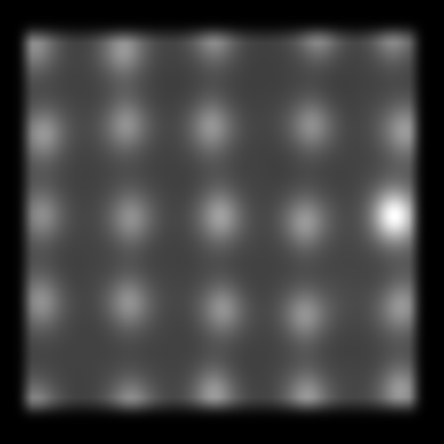
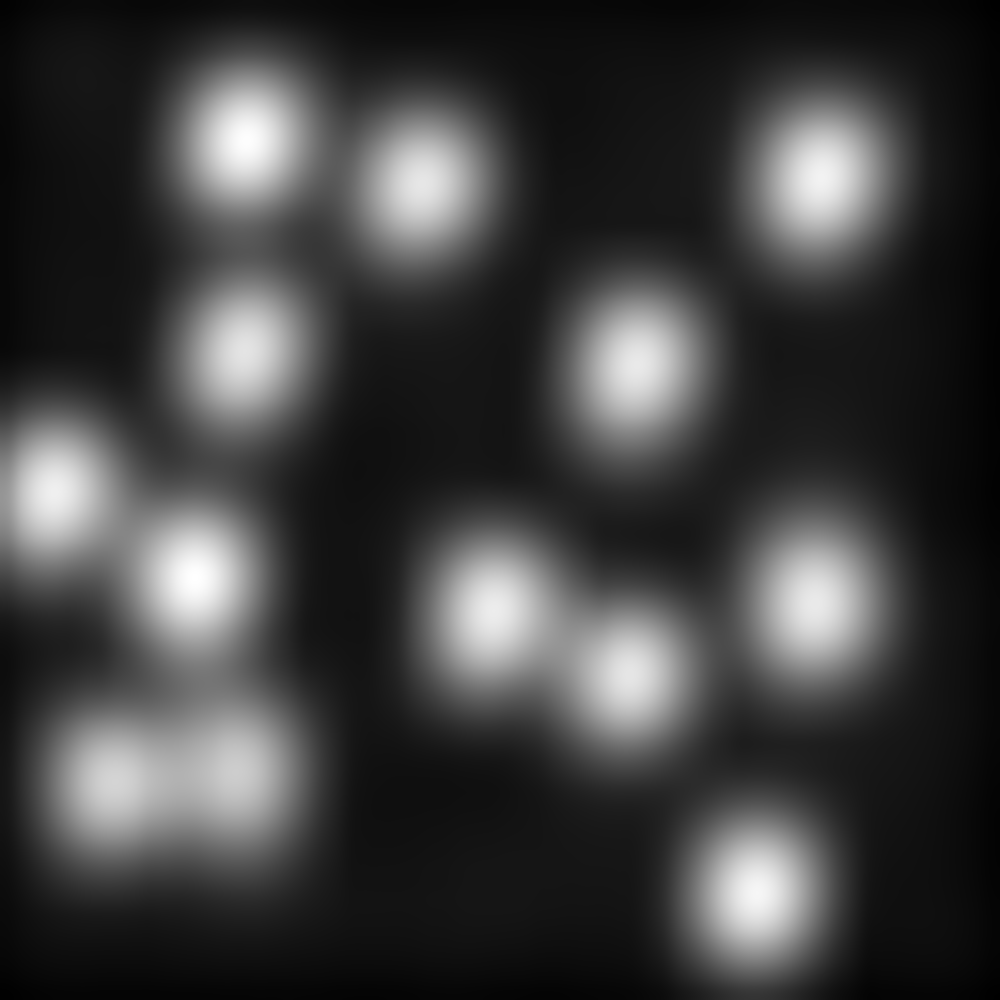
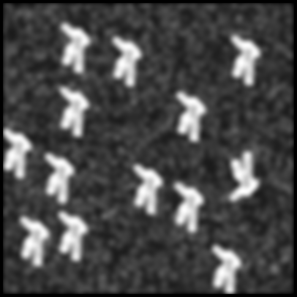
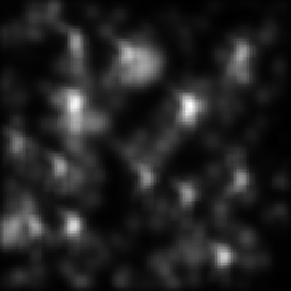
and here are the example stimuli under blur degredation:

SMILER Setup in MATLAB

Step 1.) In order to run this example, you need to have SMILER set up on your system. Code for SMILER can be found on the project page on GitHub.

If you are new to using Git, follow these instructions for checking out a Git repository for Windows, Mac, or Linux. Note that for Windows users, you may need to set up Git Bash first. An alternative would be to download the repository as a zip file, but cloning the repository allows a user to keep their SMILER software up to date with any bug fixes or other code changes.

Step 2.) In order to enable access to SMILER tools in the MATLAB environment, SMILER files need to be added to the MATLAB path. Navigate the MATLAB working directory to the smiler_matlab_tools subdirectory found in your local copy of SMILER. In the MATLAB command window, execute the following command:

>>iSMILER

This will add all SMILER files to your MATLAB path for this particular session of MATLAB. If you want SMILER to be available for all future sessions as well, you can instead call the command as:

>>iSMILER(true)

Note for Linux users: you may find yourself unable to permanently add SMILER files to the path, and instead after executing the iSMILER(true) command may find yourself receiving this warning (or one very similar to it, depending on your MATLAB version):

Warning: Unable to save path to file '/usr/local/MATLAB/R2018b/toolbox/local/pathdef.m'. You can save your path to a different location by calling SAVEPATH with an input argument that specifies the full path. For MATLAB to use that path in future sessions, save the path to 'pathdef.m' in your MATLAB startup folder.

This warning is due to the fact that by default you may lack the necessary permissions to modify the MATLAB path. The easiest way to fix this problem is to give yourself those permissions. Find your MATLAB root path by executing the command:

>>matlabroot

in your MATLAB command window. To modify the permissions of your pathdef.m file, open a terminal and execute the command:

sudo chown [user] [matlab root path]/toolbox/local/pathdef.m

You should now be able to make permanent changes to your MATLAB path.

Experiment Setup

Step 1.) Support code and stimuli images for this example can be obtained through the GitHub repository for example code.

Step 2.) To check that SMILER is correctly set up for your current MATLAB session, type the following command into your MATLAB command window:

>>which iSMILER

If SMILER is correctly configured for your current MATLAB session, this should return the path to your local copy of the iSMILER.m file. If instead the command returns:

'iSMILER' not found.

then SMILER has not been correctly added to your MATLAB path, and you should follow the instructions in Step 2 of the previous section.

Step 3.) Navigate your MATLAB working directory to your local code subdirectory of the SMILER_MATLAB_example repository. This folder should contain several functions as well as the noise_example.m script. This file contains all the necessary steps to execute this experiment.

Experiment Walkthrough

Although it is possible to simply execute the example experiment by running the noise_example script, this section will walk through the script code and explain in more detail the choices and behaviours of the experiment.

There are three main sections to the code:

1. Initialization
2. Main Loop
3. Plotting Results

Initialization

The first initialization step is to create a list of the paths to the images we want to process. Note that the code I've used to do this is a quick hack which makes three major assumptions: all input images are located in a folder which is found along the relative path ../images/stimuli/ from the current working folder (where the example script is found), the contents of this folder only consists of images which we want to process, and the names of those images are such that the first two items returned by the MATLAB dir function are the . and .. folder navigation elements. If any of these assumptions become invalid, this code will likely error (or at the very least behave unexpectedly).

imlist = dir('../images/stimuli/');
imlist = imlist(3:end);

The first line finds all the contents of the folder, and the second trims off the first two elements found (the folder navigation elements).

Once we have the image set ready for processing, we want to decide which saliency models to run on those images. This line creates a cell array of model identifiers used by SMILER:

models = {'AIM', 'FES', 'GBVS', 'IMSIG', 'RARE2012'};

For the purposes of this experiment, we have chosen to use Attention by Information Maximization (AIM) by Bruce and Tsotsos, Fast and Efficient Saliency (FES) by Tavakoli et al., Graph Based Visual Saliency (GBVS) by Harel et al., Image Signature (IMSIG) by Hou et al., and Rarity-based Saliency (RARE2012) by Riche et al. However, this experiment could easily be adjusted to use a different set of models by changing this declaration. If a user would like to see which models are available in the MATLAB environment, run the following in the command window:

>>smiler_info()

This will output both a list of available models as well as information on the set of global parameters available to modify model execution. At the time of this writing, the set of models currently available consists of:

• AIM Attention by Information Maximization
• AWS Adaptive Whitening Saliency
• CAS Context Aware Saliency
• CVS Covariance-based Saliency
• DVA Dynamic Visual Attention
• FES Fast and Efficient Saliency
• GBVS Graph-Based Visual Saliency
• IKN Itti-Koch-Niebur
• IMSIG Image Signature
• LDS Learning Discriminative Subspaces for Saliency
• QSS Quaternion-Based Spectral Saliency
• RARE2012 Rarity-based Saliency
• SSR Saliency Detection by Self-Resemblance
• SUN Saliency Using Natural Statistics
• gaussian Centered Gaussian Model

To find out more information for any specific model (including citation information), you can call smiler_info with the SMILER identifier for that model. For example, to get more information about the AIM model, execute the following command:

smiler_info('AIM')

which outputs:

************************************************************
******** AIM: Attention by Information Maximization ********
************************************************************
Model citation information:
N.D.B. Bruce and J.K. Tsotsos (2006). Saliency Based on Information Maximization. Proc. Neural Information Processing Systems (NIPS)
The following parameters are available for the AIM model:
AIM_filters
Default value: 21jade950.mat
Valid values: 21infomax[900,950,975,990,995,999].mat, 21jade950.mat, 31infomax[950,975,990].mat, 31jade[900,950].mat
Description: The feature filter set to be used by the AIM algorithm. In the form [size][name][info], where each filter is size by size in dimension, name is the ICA algorithm used to derive the filters, and info provides a measure of the retained information (higher numbers correspond to more filters).

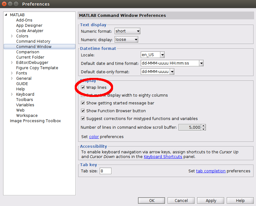
Note that for display purposes, we recommend users have the 'Wrap Lines' option turned on for their command window, as this will make the output of smiler_info much more readable. This should be found in a similar location for most versions of MATLAB; in version 2018b, for example, it is found under the Display settings of the Command Window tab (circled in red in this image:)

Getting back to the experiment script, the next several lines of code construct a set of function handles corresponding to the model identifiers stored in the cell array we just constructed. Note that if you want to use SMILER in MATLAB, these next few lines represent one of the most useful code patterns to learn and understand, and I highly recommend incorporating them into your own experiment scripts.

modfun = cell(length(models),1);
for i = 1:length(models)
  modfun{i} = str2func([models{i}, '_wrap']);
end


Following the execution of this loop, the ith element of modfun is now a function handle which points at the SMILER wrapper for the ith model included in the models cell array. A function handle lets you invoke the function pointed to by that handle, and dynamically constructing an array of function handles allows us to easily and programmatically adjust which models are being run by a given script. Example code for using these function handles is provided in the main loop section.

After setting up function handles it is important to decide what parameters we want to set for our experiments. In this example, we are going to run each individual model with its default settings with one exception. Since we know we are operating over search arrays which do not have a spatial prior for the target location, we would like to eliminate overt spatial biasing in the models being tested. We do this by setting the global SMILER center_prior parameter to none.

params = struct();
params.center_prior = 'none';

The steps described above provide a common template for how to set up a SMILER experiment in a MATLAB script. The details (such as which images are to be processed and which models are to be run with what parameter settings) may vary, but the basic pattern of usage will largely stay the same. The next lines are more specific to this example, and so will only briefly be described here.

A brief note on the experiment design: this example experiment investigates the ability of a saliency model to detect a singleton target in a search array under the presence of noise degredation. The most common saliency metrics are based on human fixation prediction, which is not applicable to this test. Salient object detection metrics may be closer in appropriateness, but their reliance on a binary target mask may be inappropriately strong. After all, distractors are called that because they may distract an observer. We therefore do not necessarily want the distractors to be assigned zero salience, but rather simply would like to see the target receive a higher salience value than the distractors.

As part of this comparison, we need to determine which pixels belong to the target and which pixels belong to the distractors. Target and distractor masks are provided as part of the experiment, but it is possible that a saliency algorithm may assign high salience to a nearby pixel outside of these bounds due to the nature of kernel convolution mechanics or image resizing errors. To try and reduce these errors, the dilation constant dil dilates the target and distractor masks; this value may be adjusted if the user would like to explore how accurately the maximum salience of a scene element is assigned relative to its tightly bound mask.

The pointprops and blurprops arrays control which noise settings will be tested for point noise and blurring, respectively. Arrays to store the ratio of maximum target and distractor salience values are initialized in point_results and blur_results. The flag variables provide user control over image logging; if flag_save_examples is set to false, then no images will be saved during the execution of the example script. If it is set to true, then images will be logged at the location specified in output_path for the noise settings specified by flag_point (for point noise) and flag_blur (for blurring noise).

After determining these final settings, it is now time to run the example.

Main Loop

The example experiment consists of a main outer loop which iterates through the input images (in this case, just two). In this outer loop an image is loaded into memory along with the corresponding target and distractor masks, which will be used for saliency map score calculations.

Each noise condition has a corresponding internal loop. The structure of these loops is identical save for the type of noise applied, so only the point noise loop will be explored here in detail. Note that both the pointnoise and blurnoise functions provided are custom to this example and are not standard MATLAB functions. You can find more information about them in their respective .m files or by calling in the command window:

>>help pointnoise

or

>>help blurnoise

Once the image has been degraded by noise, a final internal loop iterates through the saliency models being tested in this experiment to calculate the corresponding saliency map and evaluate the ratio between assigned target and distractor salience values. The line:

salmap = modfun{k}(testimg, params);

uses the function handles previously populated in the modfun array to execute the SMILER saliency wrapper for the kth saliency model being tested with the input arguments testimg (the current noise-degraded input image) and params (which in this case only contains the user-specified setting to turn off center-prior calculations, and will otherwise be populated by default values for each model). The following line:

point_results{k}(i,j) = maxrat(salmap, targmap, dil, distmap);

executes the custom metric used in this example for calculating the ratio of the maximum salience assigned to a target pixel to the maximum salience assigned to a distractor pixel. Note that, as with any performance metric, this method of evaluation carries with it a number of assumptions and simplifications, but for the purposes of an example I felt it was an adequate and interesting calculation.

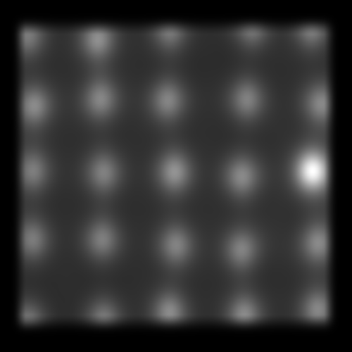
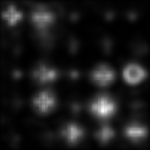
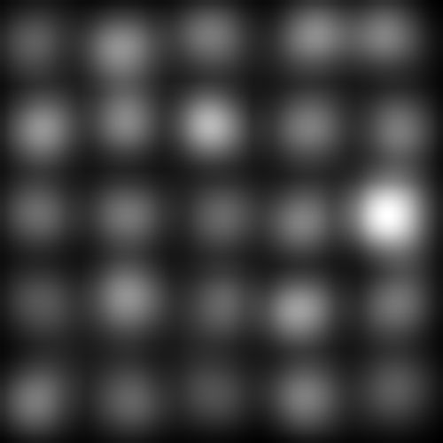
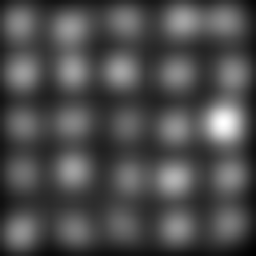
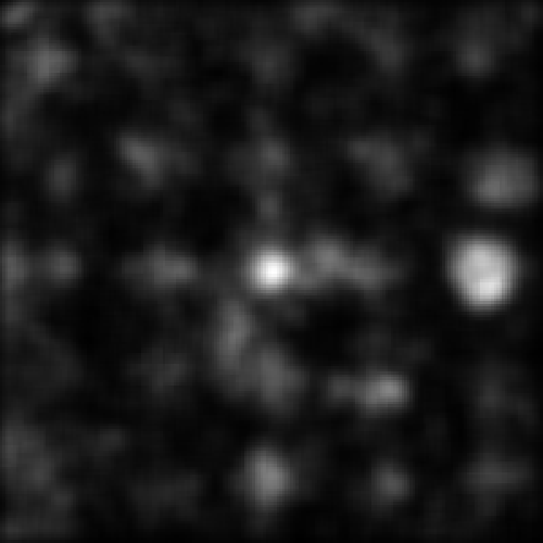
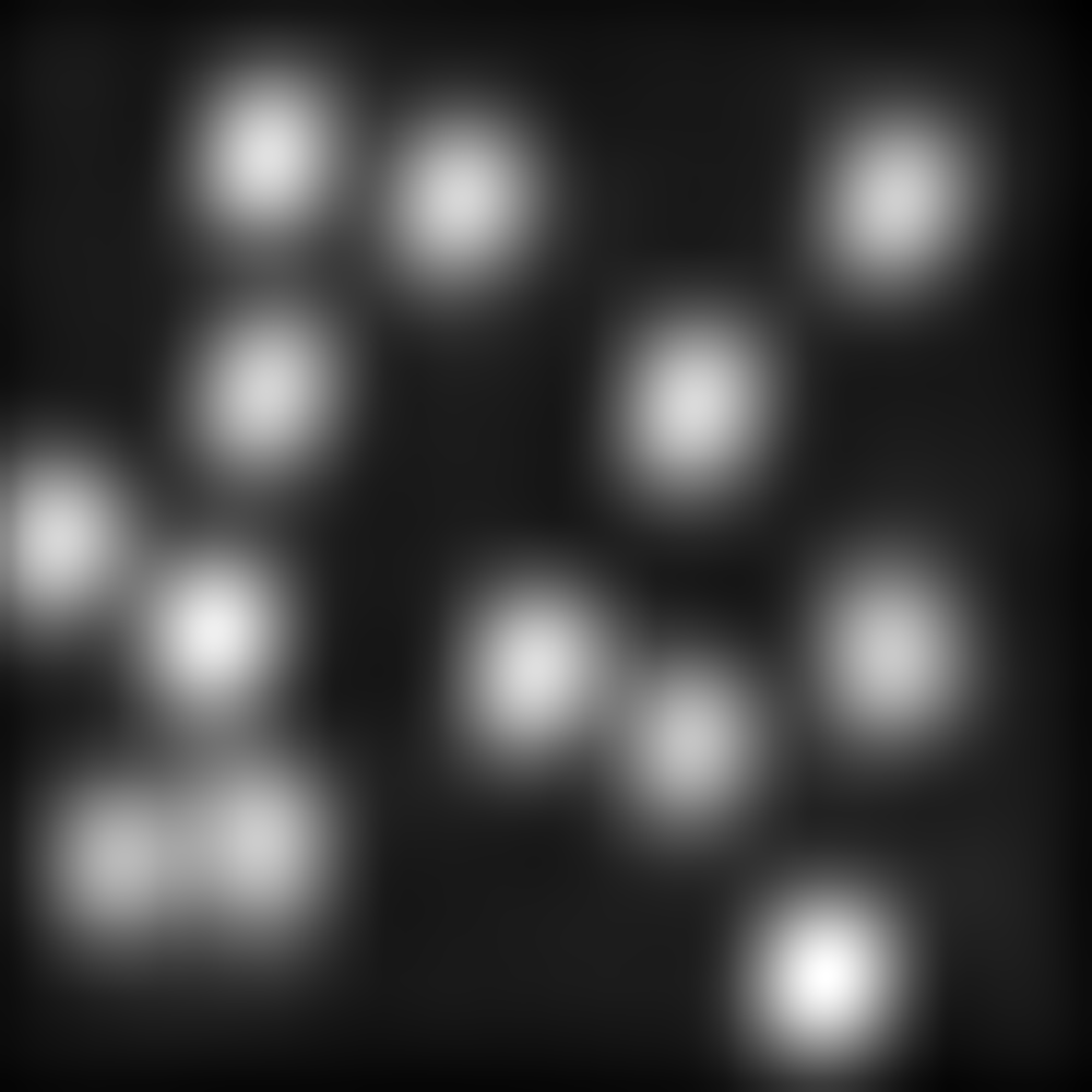
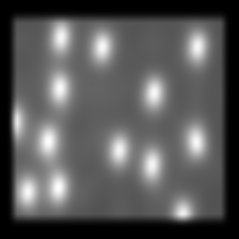
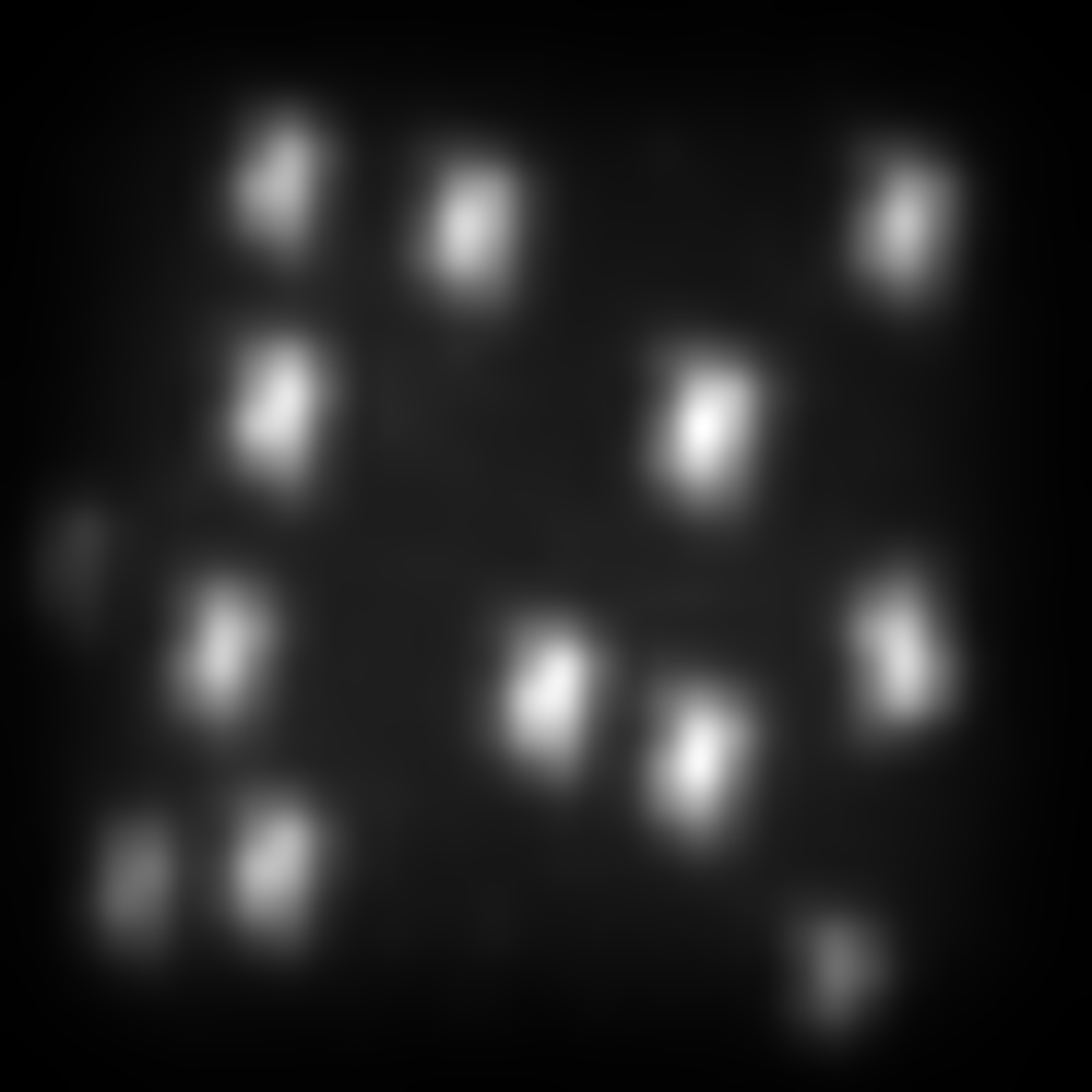
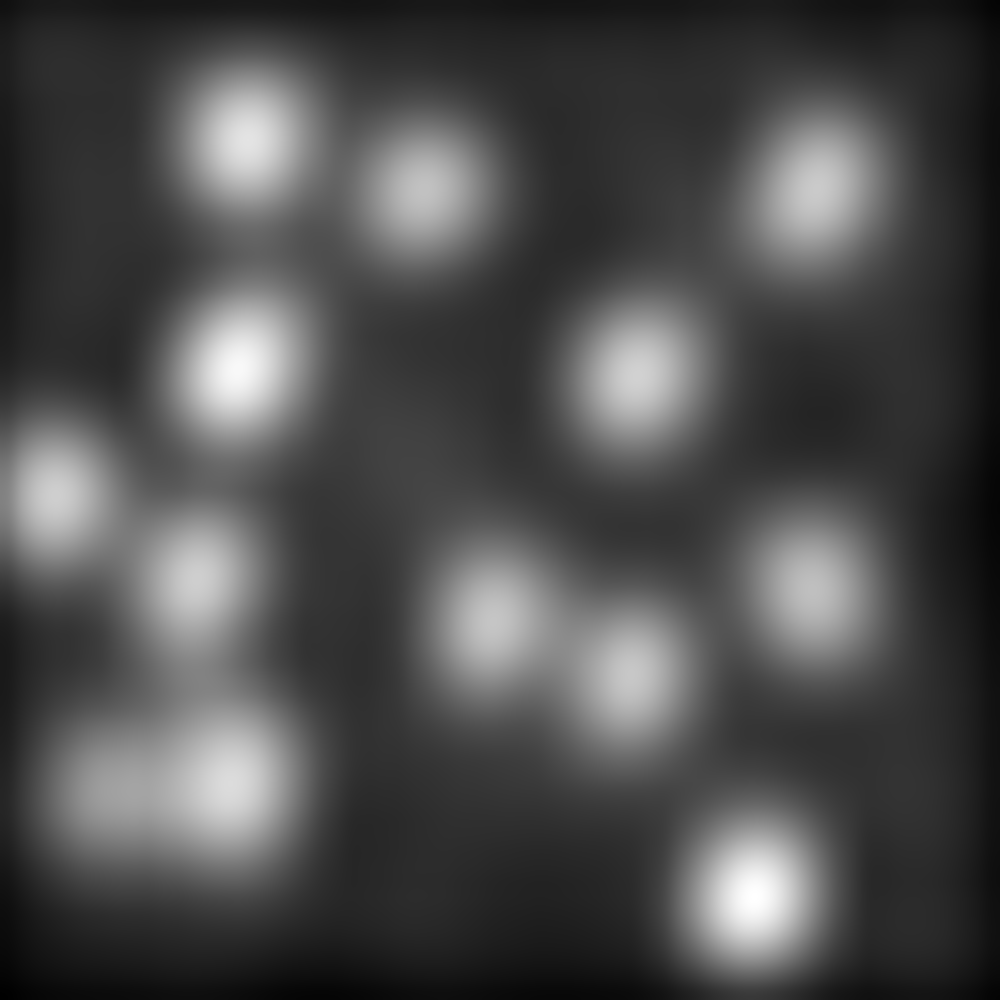
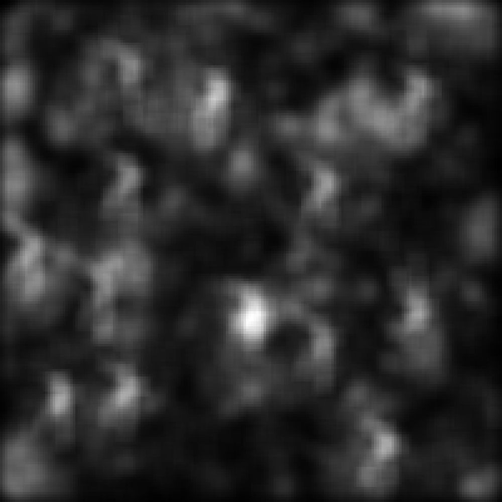
The remaining loop elements simply check to see if this loop iteration corresponds to one for which output images should be saved. Example output is shown below for the point noise settings which are provided in the default experiment script:

Plotting Results

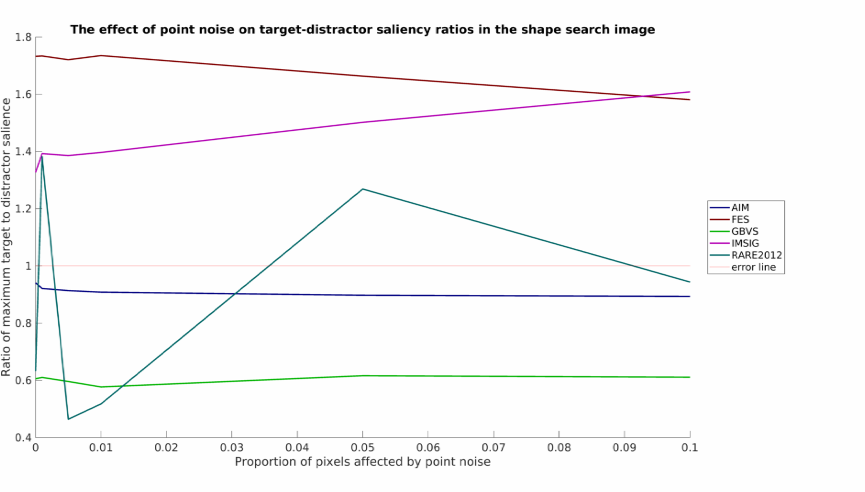
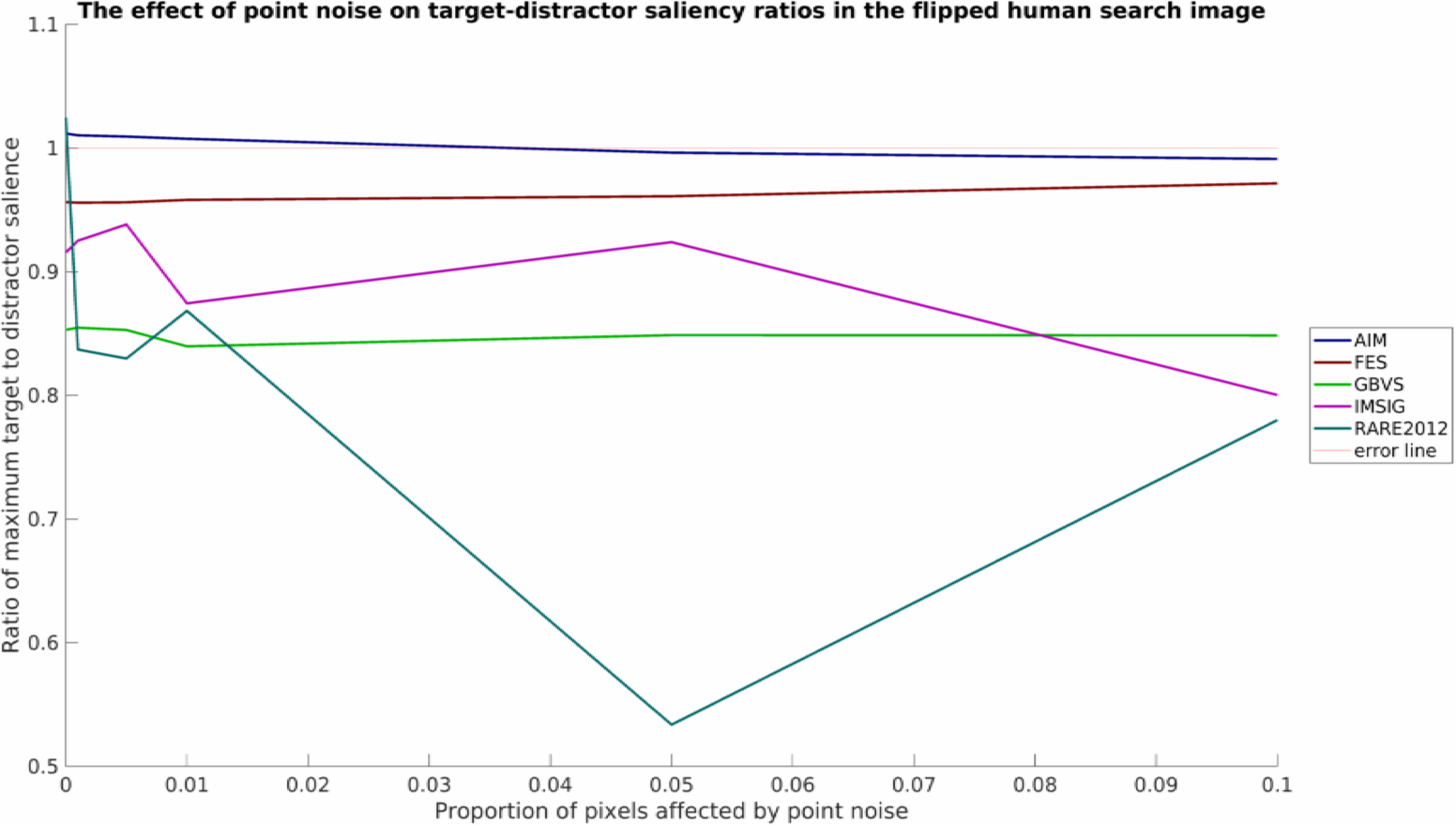
The final section of the example experiment script plots output, producing a set of performance graphs. These include output for the point noise stimuli:

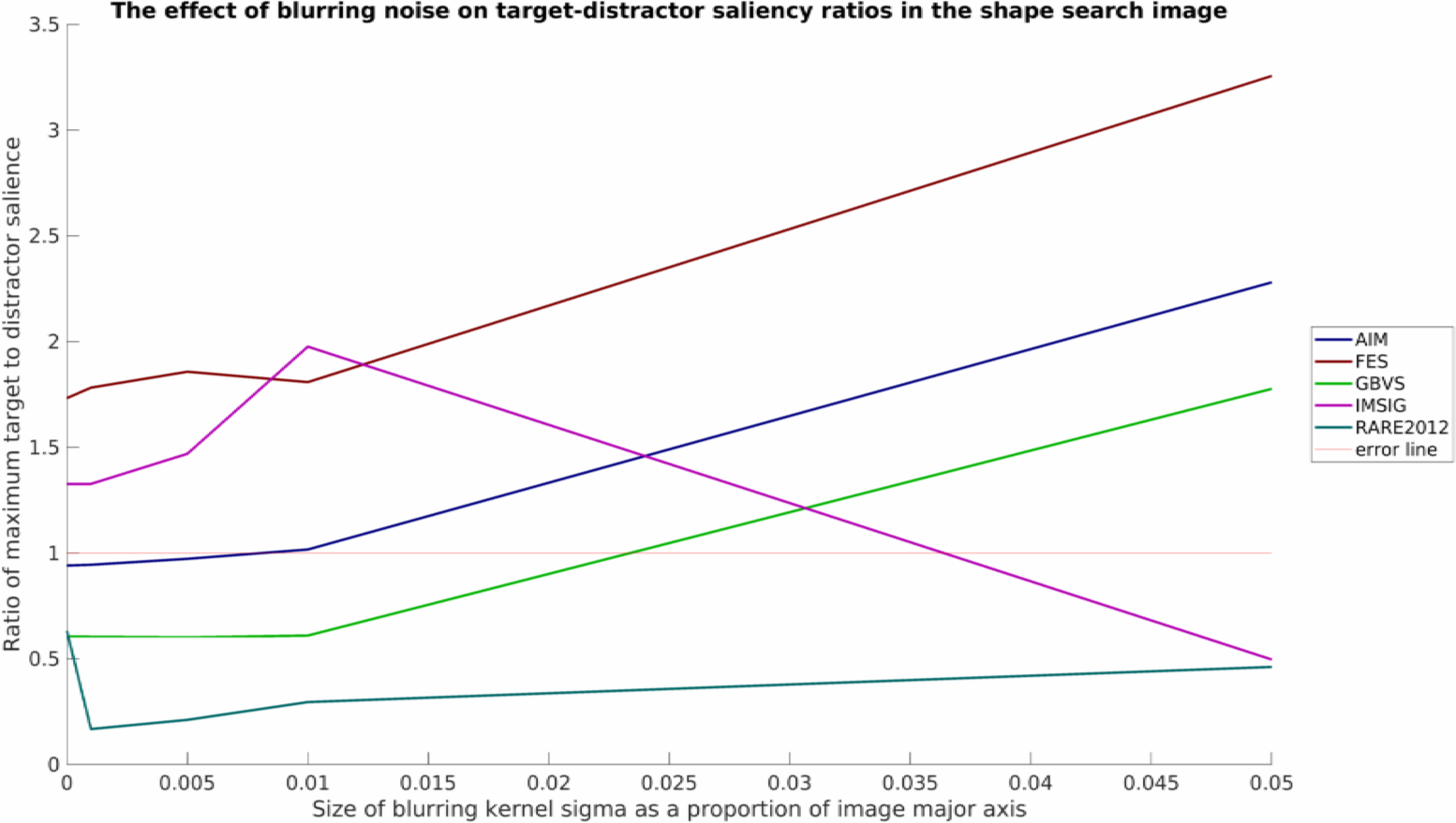
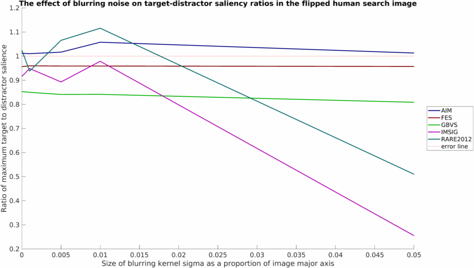
and for the blurred stimuli:

Note that all plots here have also been processed by myaa and saved using export_fig, both highly useful third-party plotting tools for MATLAB.

Concluding Remarks

As was mentioned, this is a relatively simply toy example with limited data, but nevertheless some interesting patterns can be seen. It would appear that none of the models tested work well in all conditions. RARE2012 seems particularly vulnerable to point noise, whereas IMSIG is similarly vulnerable to blurring (though not too heavily affected by point noise). Interestingly, blurring appears to have a beneficial affect for many of the models over the shape stimuli, while producing a neutral or detrimental effect in the flipped human example.

Overall, this example is meant to showcase SMILER's use for rapidly setting up batch processing to produce a set of saliency maps for analysis. Regardless of the application or goal of your saliency research, we hope that this example can provide a guide for use.