SMILER CLI Example: Singleton Target Saliency
Images and code to run this example can be downloaded from this GitHub repository.
Introduction
This is an example which showcases how to use SMILER's command line interface (CLI). Note that when MATLAB is available on a system the SMILER CLI can be used to support MATLAB-based models using the MATLAB engine for Python, but this example experiment is designed to use only non-MATLAB models to ensure access to those without an available license for MATLAB. For more information about installing and running the MATLAB engine for Python, see the official MATLAB documentation and the information provided in the SMILER readme.
Note that this exercise is designed purely as an example; the stimuli and experiment design have been selected to show an interesting use case for saliency models, but the size of the test is purposefully kept small to run in a reasonable amount of time. Any conclusions or judgements about algorithm performance are therefore tentative at best.
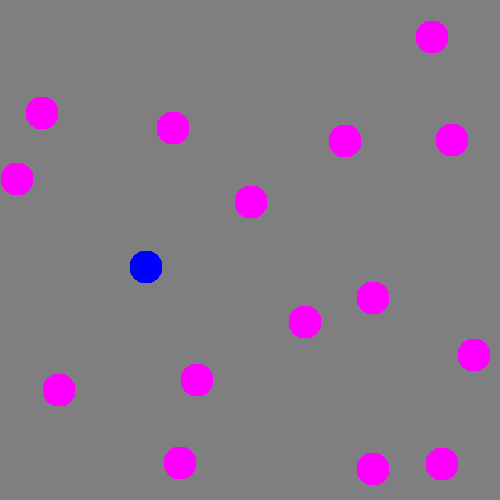
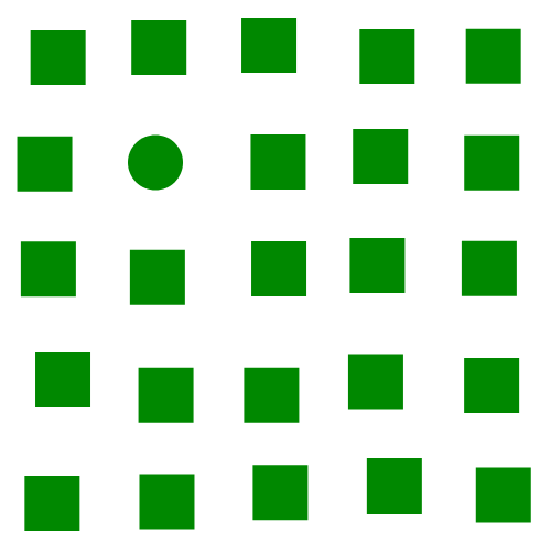
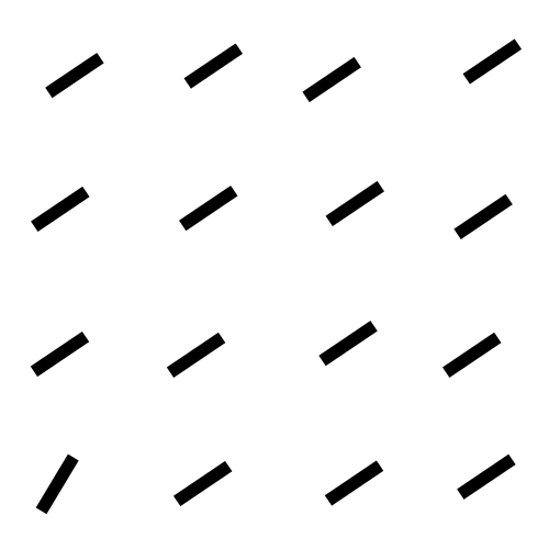
The focus of this example is on singleton search targets in psychophysical search arrays. Each search array contains a single unique target which contextually would be expected to be found to be more salient than other elements in the image. This experiment examines how this judgement of target salience changes with the type of feature defining the singleton: colour, shape, orientation, or size.

SMILER Setup
In order to run this example, you need to have SMILER set up on your system. Code for SMILER can be found on the project page on GitHub. Note that at this time the SMILER CLI is only supported for Linux operating systems, and has been tested under Ubuntu 18.04 and Ubuntu 16.04. If you want to get it working under a different operating system, you are encouraged to contribute any necessary changes to the project to increase support.
If you are new to using Git, follow these instructions for checking out a Git repository on Linux. An alternative would be to download the repository as a zip file, but cloning the repository allows a user to keep their SMILER software up to date with any bug fixes or other code changes.
Once SMILER has been cloned or extracted, it is necessary to install its prerequisites. Information for doing so, as well as some helpful optional steps, can be found in the Installation section of the project readme.
Experiment Setup
Step 1.) Support code and stimuli images for this example can be obtained through the GitHub repository for example code.
(Optional) Step 2.) If you have configured SMILER to be part of your environment, you can check that it is available using the terminal command:
$ which smiler
If SMILER is correctly configured, you should receive as output the path to your local copy of the smiler executable. If not, SMILER can still be run by navigating to the containing folder and running SMILER from there.
To run SMILER using the CLI, we recommend creating a YAML experiment file for each experiment you would like to execute. This not only provides a human-readable record of all settings used, but also allows for easy sharing of experiment specifications between research groups for rapid replication of results. This example experiment is specified in the file smiler_psych.yaml. An annotated image of the file is shown below, explaining the different parts:
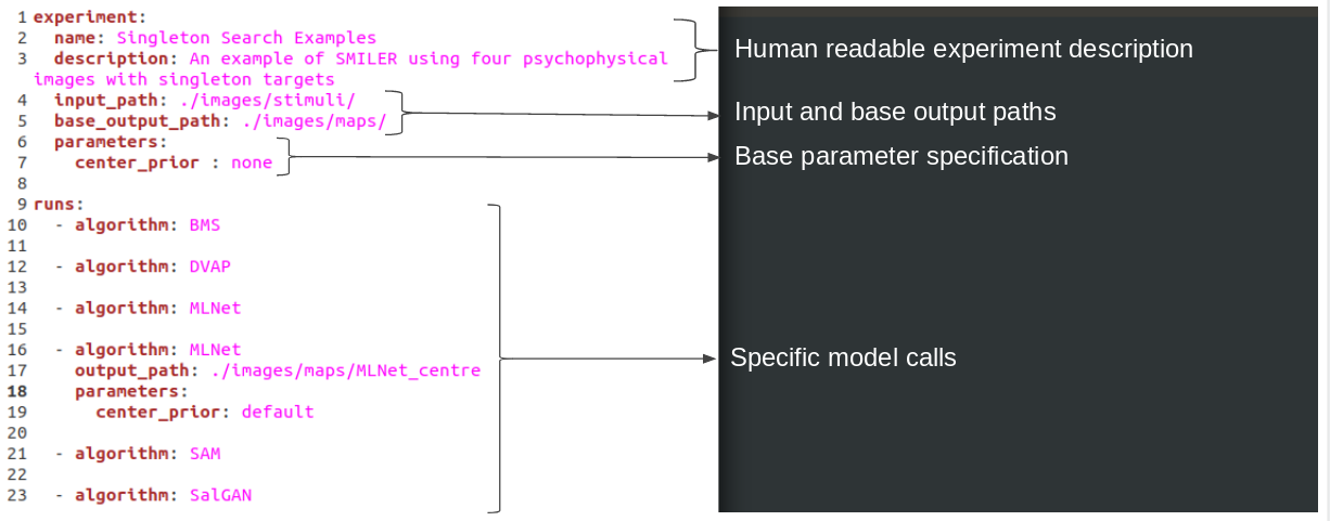
Note that each experiment file consists of a set of base parameters specified at the top of the file as characteristics of the "experiment" environment, and then each model execution is encapsulated in a separate "run". Input and output paths are always specified relative to the YAML file. Each run will inherit the base parameters specified by the experiment unless specifically told to override those results; in this experiment, all models are being run with the center_prior parameter set to none with the exception of one MLNet run which instead uses the default parameter. This allows us to examine how strongly the built-in center biasing of MLNet affects its performance on stimuli like psychophysical search arrays which do not have an inherint bias toward the center. Note that it is also necessary to specify a new output path for this MLNet run, otherwise it will conflict with the MLNet executed beforehand.
Of course, this is not an exhaustive list of models available in SMILER, and you could run a much more extensive experiment if you wish. If you want to extend the experiment file with more runs, you can see a list of available models using the command:
$ smiler info
which, at the time of this writing, will output the following list:
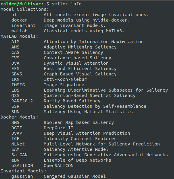
Note that the models are split into three groups: MATLAB Models, Docker Models, and Invariant Models. The MATLAB models, even when run through the CLI, require the MATLAB python engine to be configured for a valid installation of MATLAB (see the Installation section of the project readme for further information). The Docker Models, conversely, are only available through the SMILER CLI. In consideration of those who do not have MATLAB available, this example uses only models from this second set. The final, Invariant Models, provides models which output a map independent of the visual appearance of the input image. At the time of this writing there is only one such model, gaussian, and it will output a Gaussian center prior which is scaled to the dimensions of the input image. For a dataset with consistent input image sizes, therefore, we would recommend only running it once to save processing time.
To find out more information for a specific model (including citation information and model-specific parameters), you can call $ smiler info [MODEL], where [MODEL] is replaced by the SMILER identifier for the specific model in question. To see a list of global parameters shared by most or all models (such as the center_prior parameter featured above), run the command $ smiler info -p. For example, to get more information about the BMS model, execute the following command:
$ smiler info BMS
which outputs:
      ************************************************************

      ************ BMS: 'Boolean Map based Saliency' *************

      ************************************************************


      Version: 1.1.0


      Citation: Zhang, Jianming, and Stan Sclaroff. "Saliency detection: A boolean map approach." Proceedings of the IEEE international conference on computer vision. 2013.


      Path: /home/calden/Documents/Work/SMILER_release/models/docker/BMS


      dilation_width_1

          Default:      7


      dilation_width_2

          Default:      9


      max_dim

          Default:      400


      sample_step

          Default:      8


      whitening

          Default:      True


      Notes: This model's code has been built as part of the docker image. If you modify it, use the Dockerfile.BMS to build a new docker image locally.
Running the Experiment
Once you are satisfied with the YAML file, you can run it using the command:
$ smiler run -e [PATH_TO_YAML]
Therefore, if you have SMILER set up to provide system-wide calls, you can navigate to the folder containing the YAML file and execute:
$ smiler run -e smiler_psych.yaml
or, if you don't have system calls available for your installation of SMILER, you can navigate to the folder containing SMILER and execute the command with smiler_psych.yaml replaced by the full path to your experiment file. Note that regardless of the current path when making the execution call, all input and output paths for a given YAML file are interpreted relative to that YAML file, so pathing will remain consistent.
One final note: each docker model tends to have some overhead associated with initialization, which means that running this small batch of experiment images will take several minutes, or possibly longer if this is your first time executing a given docker model as the docker image for that model will need to be downloaded.
Results
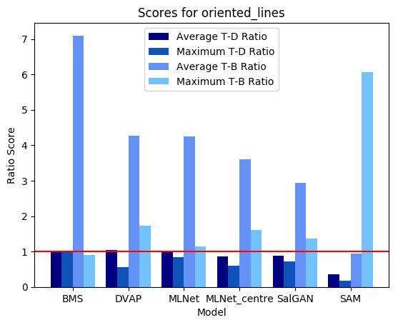
Calculating performance on these types of images is not necessarily straightforward, as standard fixation metrics do not apply. This example provides for convenience a few metrics based on saliency ratios; these metrics compare either average or maximum saliency values over the target versus distractor pixels (T-D) or over the target versus background pixels (T-B). Note that the values calculated below dilated target and distractor masks by 2 pixels in order to compensate for small localization errors on the part of the saliency models.
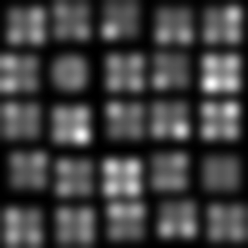
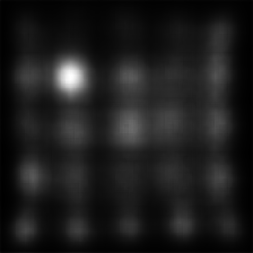
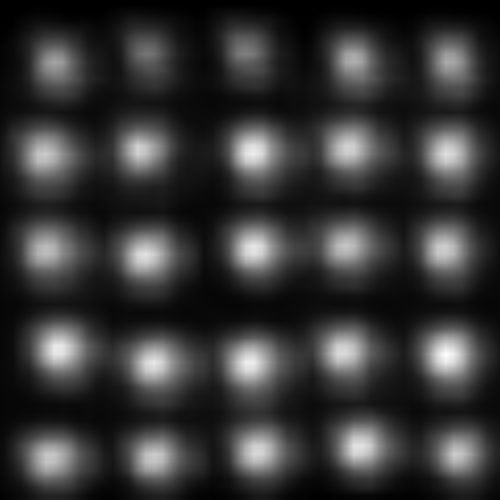
Shown below are results produced for each image for the set of models used by default in this example (note that for space considerations when displaying maps MLNet is only shown for output which does not include centre bias). All score plots include a red line; any values falling below this line indicate a ratio less than one which indicates a major error.

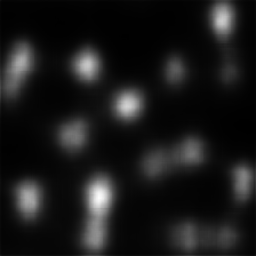

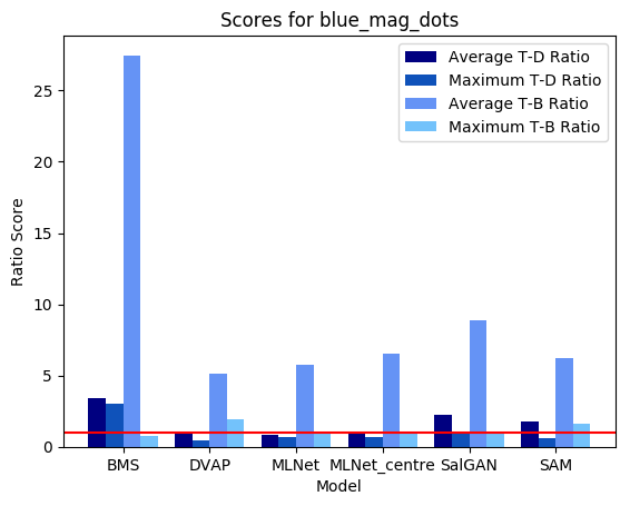
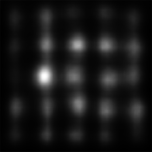
We can see that on a whole, BMS does a very good job of highlighting the blue singleton target, as well as further differentiating between the magenta distractors and the background. However, the fact that the bright blob of salience assigned to the target spills over into the background causes the Maximum T-B ratio metric to register an error for BMS. This is arguably an issue with the metric; depending on the application, it may or may not be important to accurately localize salient pixels. By an large, though, we can see that all four deep models tested struggle much more with this task; SAM and SalGAN are both able to highlight the target as more salient on average than the distractors, but SalGAN highlights a handful of distractors as roughly equivalent in saliency, and SAM finds the central distractor to be distinctly more salient, even if the peripheral distractors bring the overall distractor average below that of the target.
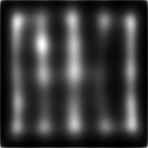
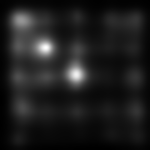
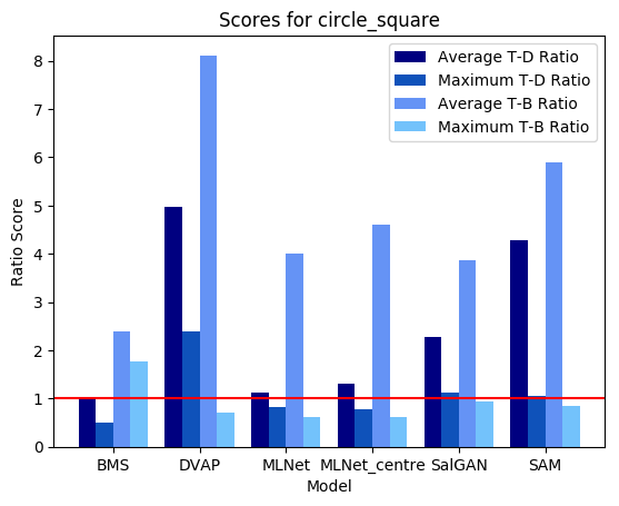
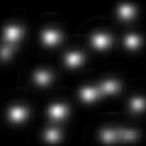
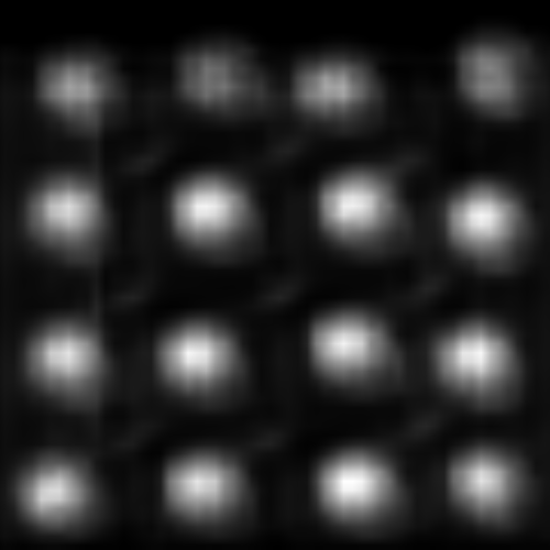
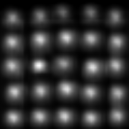
Where BMS was the standout performer in the example image above, here we see that it really struggles with detecting the shape singleton, and instead has a tendency to mark the corner elements of several of the square distractors as the most salient elements in the image. In turn, DVAP, which performed very poorly for the colour singleton, does a remarkable job in isolating the circle singleton here. MLNet struggles to differentiate between target and distractor, though it does clearly segment scene elements from the background. SalGAN, by contrast, moderately highlights the circle target but registers a number of odd background striations. Like with the previous example, SAM does a good job of highlighting the target on average, but also puts a heavy emphasis on the most centrally located distractor.

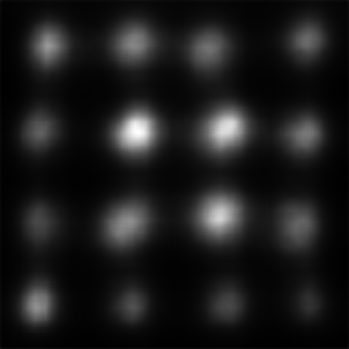
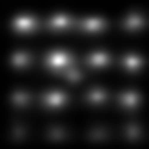
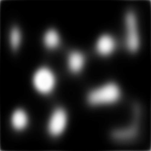
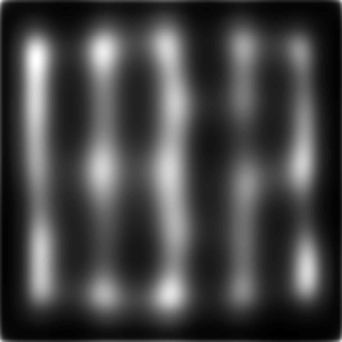
Overall, this example image was the most difficult for the models tested here. No model did very well in highlighting the target. BMS segmented search array elements from the background rather well, but could not distinguish the singleton target from the surrounding distractors. SalGAN, again, showed some odd striation artifacts. SAM had the worst performance, in part perhaps the target was in the corner of the image and SAM includes an integrated, learned center bias which cannot be removed by SMILER (unlike an explicit post-processing bias step such as the one used by MLNet).

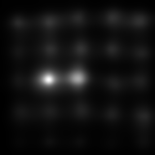

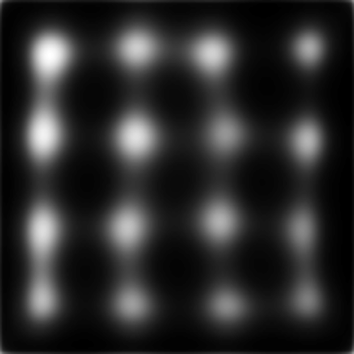
DVAP and SAM both highlight the target, though SAM still seems to be heavily affected by the spatial bias and may not have successfully found the target had it been further from the image centre. MLNet, despite explicitly utilizing features in a multi-scale manner, fails to highlight the target. BMS, also, segments search elements from the background but does not distinguish target from distractor.
Concluding Remarks
This is a relatively simply toy example with limited data, but nevertheless some interesting patterns can be seen. It would appear that none of the models tested work well in all conditions, and overall saliency models based on deep neural networks have difficulty with this style of stimulus.
This example is meant to showcase SMILER's use for rapidly setting up experimental runs to produce a set of saliency maps for analysis. Regardless of the application or goal of your saliency research, we hope that this example can provide a guide for use.